$\phi$ nodes in SSA [1-3] allow to connect multiple definitions of a value from different basic blocks. They are, by definition, non-deterministic: one of their values will be arbitrarily picked, depending on how the CFG runs. When lowered to the assembly, they are associated to a memory region: if an operation modifies an input value of such a node, then the value is written in memory; when you need the output of a $\phi$, you read from that same memory location.
In the 90’s, some authors [8] thought about the possibility of associating some boolean conditions to each input of a $\phi$ node, so that it is easier both to interpret the code and to optimize it, since you are always well-aware of the conditions which force one specific usage.
The authors ended up distinguishing two different types of $\phi$ nodes:
-
$\mu$ nodes are loop-headers. They are in charge of picking the value from the outside of the loop both at the first execution and after every loop batch is terminated. They have two inputs only, the outside value and the regenerated one. You pick the latter when the loop-exit condition is false.
-
$\gamma$ nodes are if-then-else statements. They have two inputs and a simple boolean condition which tells the correct value to be used. A single $\phi$ can be made using a tree of these nodes, making sure that a value is generated whenever their correspondent conditions are true.
This representation was seldom adopted in literature, since, in the compiler world, the SSA gates are more than enough. However, recently some authors [11] tried to exploit it, especially in the context of HLS (High Level Synthesis) [4]. Hardware needs to be deterministic, thus it can be convenient to have some boolean conditions associated to each $\phi$ node.
Many translation mechanisms from SSA to GSA are available in literature [3, 6, 8-10]. Some of them start from a pre-SSA format, to obtain an IR that is already compliant with the standard. Others prefer adding some boolean conditions to each already-existent $\phi$.
The following section shows a methodology to obtain these same conditions out
of pre-existent SSA nodes. This methodology works as expected, but it has no
formal proof. When designing it, Polygeist was utilized as frontend. The
method was developed over the cf dialect in MLIR [5], so that some implicit
$\phi$ nodes are provided in the form of block arguments. It is reasonable to
believe (again, without formal proof) that the methodology only works on
reducible CFGs. Out of the multiple tests that have been done, no irreducible
graph was obtained out of Polygeist.
The reader should be familiar with the following concepts: dominance tree [12], control dependency graph [7].
From $\phi$ gates to $\mu$ gates
The following conditions determine whether a $\phi$ gate can be converted into a $\mu$ gate:
- The $\phi$ function must have exactly two inputs.
- The $\phi$ function must reside within a loop.
- The $\phi$ function must be located in a basic block that serves as the loop header.
- One input to the $\phi$ function must originate from outside the loop.
If these conditions are satisfied, the $\phi$ function is converted into a
$\mu$.
The example below shows exactly the above scenario: %1 is $\phi$(%c0_i32,
%6). It is in a loop header (made of ^bb1 and bb2), and the first value
comes from a block outside of the loop.
module {
  func.func @phi_to_mu() -> i32 {
    %c0_i32 = arith.constant      0 : i32
    %c0 = arith.constant          0 : index
    %0 = memref.load %arg0[%c0]     : memref<8xi32>
    cf.br ^bb1(%c0_i32 : i32)
  ^bb1(%1: i32):                    // 2 preds: ^bb0, ^bb2
    %2 = arith.cmpi slt, %1, %0     : i32
    cf.cond_br %2, ^bb2, ^bb3
  ^bb2:                             // pred: ^bb1
    %4 = arith.index_cast %1        : i32 to index
    %5 = memref.load %arg0[%4]      : memref<8xi32>
    %6 = arith.addi %1, %5          : i32
    cf.br ^bb1(%6 : i32)
  ^bb3:                             // pred: ^bb1
    return  %1 : i32
  }
}
From $\phi$ gates to $\gamma$ gates
The remaning $\phi$ nodes should be converted into $\gamma$ nodes. However, a single $\gamma$ has only two inputs, thus it is not enough for a multi-input $\phi$. The strategy involves creating a tree of $\gamma$ functions, each driven by a simple boolean condition (the exit condition of a basic block). The following steps outline the process to extract such a tree for any $\phi$ function.
Initialization and Input Structure
Each $\phi_i$, located in $B_{\phi_i}$, is analyzed individually. The function $\phi_i$ receives $N \geq 2$ inputs, labeled as $i_{\phi_i}^0, i_{\phi_i}^1, \dots, i^j_{\phi_i}, \dots, i_{\phi_i}^{N-1}$. Each input originates from a basic block $B_{\phi_i}^j$, indexed by $j$. All these blocks share a common dominator ancestor in the control flow graph, referred to as $B_{CA}$.
Input ordering
The inputs of the $\phi_i$ function are sorted based on the relationships of their originating basic blocks. The indices are assigned such that if basic block $B_i$ properly dominates $B_j$, then $i < j$. This order does not affect the semantics of this original $\phi_i$, since this gate is, by definition, order-less. However, it helps while moving on in the algorithm.
Path Identification and Boolean Condtions
For each input $i_{\phi_i}^j$, the path with the following characteristics are identified:
- A path originates from $B_{CA}$ and terminates in $B_{\phi_i}$.
- Each path must pass through $B_{\phi_i}^j$ but must avoid $B_{\phi_i}^k$ if there exists an input of $\phi_i$ in $B_{\phi_i}^k$ such that $k > j$.
Each path $P_i$ is associated with a set of $M$ boolean conditions, $c_{P_i}^0, c_{P_i}^1, \dots, c_{P_i}^{M-1}$, representing what needs to happen in the CFG for that path to be taken. The boolean condition for a single path is expressed as:
\[c_{P_i} = c_{P_i}^0 \land c_{P_i}^1 \land \dots \land c_{P_i}^{M-1}.\]The boolean condition for the input $i_{\phi_i}^j$ is the disjunction of the conditions for all paths associated with it:
\[c_{\phi_i}^j = \bigvee_i c_{P_i}.\]Constructing the $\gamma$ Function via Recursive Expansion
The $\gamma$ functions for $\phi_i$ are constructed using a recursive expansion process, which considers one literal at a time:
- Begin with the literal with the lowest index. Use this condition as the selector for the first $\gamma$ function.
- Divide the remaining boolean expressions into two sets:
- Expressions where the literal is true; replace the literal with a true; this will become the true input of $\gamma$.
- Expressions where the literal is false; replace the literal with a false; this will become the false input of $\gamma$.
- Apply the expansion recursively to both sets, proceeding with conditions in increasing order.
- Each $\gamma$ function branches into two: one branch for true conditions and another for false conditions. If only one value remains in a branch, it is used directly as the argument of the $\gamma$ function without further expansion.
Examples
Example 1: Simple Boolean Conditions
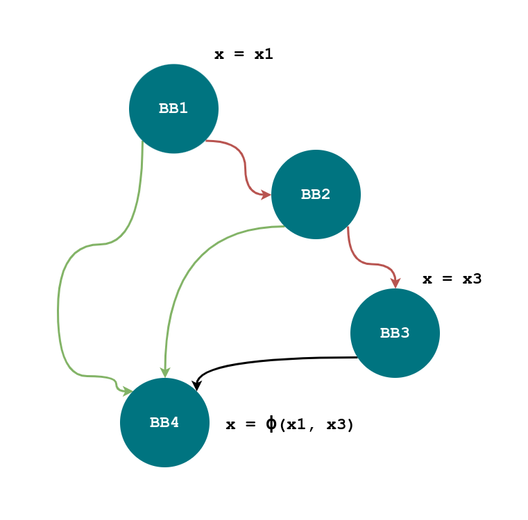
The above picture shows a CFG with a value of x modified in two
points, both in BB1 and BB3. The algorithm from the previous
example will be used to obtain a tree of $\gamma$s in place of $\phi$.
The inputs of the $\phi$ are located in BB1 and BB3. Their common
dominator ancestor is BB1. The ordering of the indices is already
correct, since BB1 dominates BB3 and $1 < 3$.
There are two paths which allow to go from BB1 to BB4 without going
through BB3: BB1 - BB4 and BB1 - BB2 - BB4. The first path is covered
with the conditions $c_1$, while the second is when with $\overline{c_1}
\cdot c_2$. For this reason, the input from BB0 is used when the following
boolean expression is true: $c_1 + \overline{c_1} \cdot c_2$.
For the other input, the boolean condition is, on the contrary,
$\overline{c_1} \cdot \overline{c_2}$.
Given the following input conditions:
\[V_1 \rightarrow c_1 + \overline{c_1} \cdot c_2 \\ V_3 \rightarrow \overline{c_1} \cdot \overline{c_2}\]The $\gamma$ tree is constructed as follows:
- Start with $c_1$. When $c_1$ is true, only $V_1$ remains, so it is the only available value, connected to the true input of $\gamma$;
- When $c_1$ is false, expand using $c_2$. If $c_2$ is true, $V_1$ remains; if $c_2$ is false, $V_3$ remains.
The resulting $\gamma$ function is:
\[\gamma(c_1, V_1, \gamma(c_2, V_1, V_3)).\]Example 2: Nested Conditions
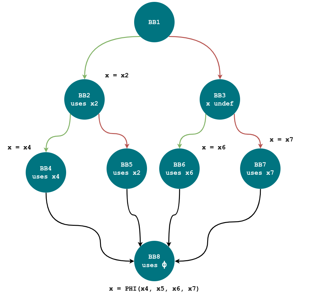
The same algorithm can be used to expand the $\phi$ in the CFG above.
It should be simple to use the path between the common dominator of each node
which defines x (BB0) until the $\phi$ basic block (BB8) to obtain the
following conditions:
The $\gamma$ tree is constructed as follows:
- Start with $c_1$. When $c_1$ is true, expand using $c_2$. If $c_2$ is true, $V_4$ remains; if $c_2$ is false, $V_5$ remains.
- When $c_1$ is false, expand using $c_3$. If $c_3$ is true, $V_6$ remains; if $c_3$ is false, $V_7$ remains.
The resulting $\gamma$ function is:
\[\gamma(c_1, \gamma(c_2, V_4, V_5), \gamma(c_3, V_6, V_7)).\]References:
[1] F. Rastello and F. Bouchez Tichadou, Eds., SSA-based Compiler Design. Cham: Springer International Publishing, 2022.
[2] K. D. Cooper and L. Torczon, Engineering a compiler. Morgan Kaufmann, 2022.
[3] R. Cytron, J. Ferrante, B. K. Rosen, M. N. Wegman, and F. K. Zadeck, “Efficiently computing static single assignment form and the control dependence graph,” ACM Trans. Program. Lang. Syst., vol. 13, no. 4, pp. 451–490, Oct. 1991.
[4] P. Coussy and A. Morawiec, Eds., High-Level Synthesis: From Algorithm to Digital Circuit. Dordrecht: Springer Netherlands, 2008.
[5] C. Lattner, M. Amini, U. Bondhugula, A. Cohen, A. Davis, J. Pienaar, R. Riddle, T. Shpeisman, N. Vasilache, and O. Zinenko, “MLIR: Scaling Compiler Infrastruc- ture for Domain Specific Computation,” in 2021 IEEE/ACM International Symposium on Code Generation and Optimization (CGO), Feb. 2021, pp. 2–14.
[6] P. Tu and D. Padua, “Efficient Building and Placing of Gating Functions,” ACMSIGPLAN Notices, vol. 30, no. 6, pp. 47–55, Jan. 1995.
[7] J. Ferrante, K. J. Ottenstein, and J. D. Warren, “The program dependence graph and its use in optimization,” ACM Trans. Program. Lang. Syst., vol. 9, no. 3, pp. 319–349, Jul. 1987.
[8] K. J. Ottenstein, R. A. Ballance, and A. B. MacCabe, “The program dependence web: a representation supporting control-, data-, and demand-driven interpretation of imperative languages,” in Proceedings of the ACM SIGPLAN 1990 conference on Programming language design and implementation, ser. PLDI ’90. New York, NY, USA: Association for Computing Machinery, Jun. 1990, pp. 257–271.
[9] P. Havlak, “Construction of thinned gated single-assignment form,” in Languages and Compilers for Parallel Computing, U. Banerjee, D. Gelernter, A. Nicolau, and D. Padua, Eds. Berlin, Heidelberg: Springer, 1994.
[10] M. Arenaz, P. Amoedo, and J. Tourino, “Efficiently Building the Gated Single Assignment Form in Codes with Pointers in Modern Optimizing Compilers,” in Euro Par 2008 – Parallel Processing, E. Luque, T. Margalef, and D. Benítez, Eds. Berlin, Heidelberg: Springer, 2008, pp. 360–369.
[11] Y. Herklotz, D. Demange, and S. Blazy, “Mechanised Semantics for Gated Static Single Assignment,” in Proceedings of the 12th ACM SIGPLAN International Conference on Certified Programs and Proofs, ser. CPP 2023. New York, NY, USA: Association for Computing Machinery, Jan. 2023, pp. 182–196.
[12] K. D. Cooper, T. J. Harvey, and K. Kennedy, “A simple, fast dominance algorithm,” Software Practice & Experience, vol. 4, no. 1-10, pp. 1–8, 2001, publisher: Citeseer.